Web and Social Network Analytics

Week 4: Unsupervised Learning Techniques

Dr. Zexun Chen

Zexun.Chen@ed.ac.uk

Feb-2026

Table of Contents

Welcome Back!

Last Week:

• Social network structure and properties
• Centrality measures (degree, betweenness)
• Community detection algorithms

This Week:

• Finding patterns in data WITHOUT labels
• Sentiment, associations, and recommendations

ShopSocial Question: How can we understand customer opinions, find product bundles, and make personalized recommendations?

Learning Objectives

By the end of this lecture, you will be able to:

1. Explain the difference between supervised and unsupervised learning
2. Apply sentiment analysis to classify customer reviews
3. Calculate support, confidence, and lift for association rules
4. Implement the A-Priori algorithm to find frequent itemsets
5. Design a collaborative filtering recommendation system

Assessment link: These techniques are directly applicable to your ShopSocial coursework analysis.

Introduction

Introduction

• Predictive Analytics:
  • All about the dependent variables
  • What if there is no dependent variable?
    • Sales purchases
    • Reviews without a score
    • Website paths
    • …

• General idea:
  • Putting similar items into a group
  • Finding features

Clustering Review

📊 Quick Poll: Customer Segments

Wooclap Question

Go to wooclap.com and enter code: RMBELP

How many distinct customer types do you think ShopSocial has?

• A. 2-3 segments
• B. 4-6 segments
• C. 7-10 segments
• D. More than 10

Clustering: The Big Idea

Think About It

You’re managing ShopSocial and want to send different marketing emails to different customer types. How would you group 100,000 customers into meaningful segments?

Clustering = Grouping similar items together WITHOUT predefined labels

• Every instance is a point in n-dimensional space
• Group based on distance: Euclidean \(d = \sqrt{\sum(a_i - b_i)^2}\) or Manhattan \(d = \sum|a_i - b_i|\)

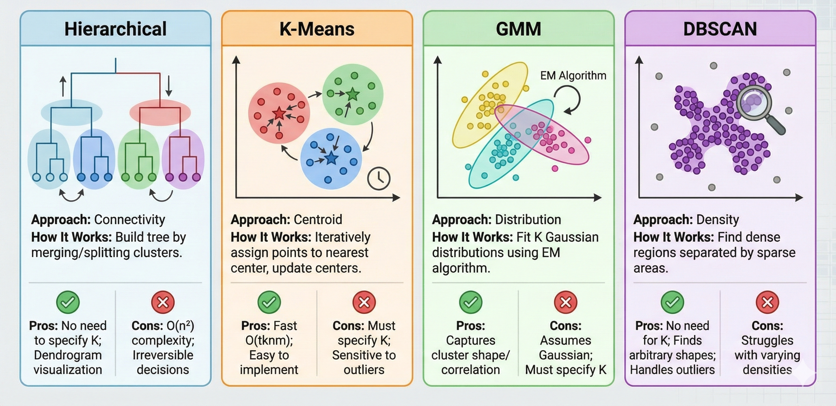
Clustering Methods: Comparison

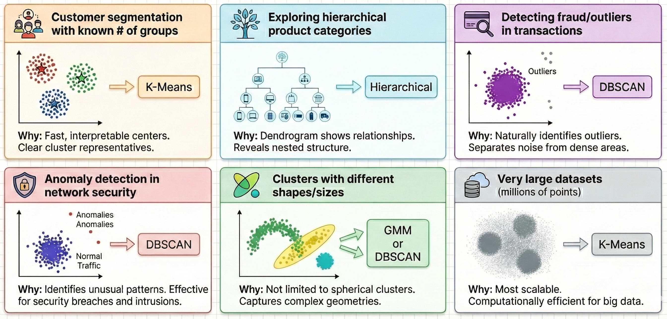
When to Use Which Method?

K-Means Visualization/ DBSCAN Visualization

ShopSocial Customer Segmentation

Using K-Means with RFM Analysis (Recency, Frequency, Monetary):

Segment	Recency	Frequency	Monetary	Strategy
Champions	Recent	Often	High	Reward loyalty
At Risk	Long ago	Often	High	Win back campaigns
New Customers	Recent	Low	Low	Onboarding emails
Hibernating	Long ago	Low	Low	Re-engagement offers

Note

Key Insight: Clustering helps ShopSocial personalize marketing without manual labeling!

Sentiment Analysis

📊 Quick Poll: Reading Reviews

Wooclap Question

Go to wooclap.com and enter code: RMBELP

When you read a product review, how quickly can you tell if it’s positive or negative?

• A. Instantly - first few words
• B. After reading the whole review
• C. Sometimes it’s unclear
• D. I look at the star rating instead

Why Sentiment Analysis Matters

Think About It

ShopSocial has 500,000 product reviews. A human reading 1 review per minute would take 347 days working 24/7 to read them all!

How can we automatically understand customer opinions?

Sentiment Analysis = Automatically determining the emotional tone of text

• Positive, negative, or neutral
• Can also detect specific emotions (anger, joy, frustration)

Sentiment Analysis Approaches

Approach	How It Works	Pros	Cons
Lexicon-Based	Count positive/negative words using a dictionary	Simple, interpretable	Misses context, sarcasm
Machine Learning	Train classifier on labeled examples	More accurate	Needs training data
Deep Learning	Neural networks (BERT, etc.)	State-of-the-art	Computationally expensive
LLM-Based	Prompt GPT/Claude/Gemini directly	Flexible, contextual	API costs, latency

Today’s Focus: Lexicon-based approach (unsupervised - no labels needed!) + LLM insights

Lexicon-Based Sentiment Analysis

Step 1: Build/Use a Sentiment Lexicon

Word	Sentiment Score
excellent	+3
good	+1
okay	0
bad	-1
terrible	-3

Step 2: Score the Text

• Sum up sentiment scores of all words
• Positive sum → Positive sentiment

Example Review: > “This product is excellent! The quality is good but shipping was bad.”

Calculation:

• excellent: +3
• good: +1
• bad: -1
• Total: +3 (Positive!)

🔍 Hands-On: Score These Reviews

Activity (3 minutes)

Using this simple lexicon, calculate the sentiment score:

Word	Score
love/great/excellent	+2
good/nice	+1
bad/poor	-1
hate/terrible/awful	-2

Reviews to score:

1. “Great product, love it!”
2. “Poor quality but nice packaging”
3. “Terrible experience, awful service”

Solutions

1. great(+2) + love(+2) = +4 (Very Positive)
2. poor(-1) + nice(+1) = 0 (Neutral)
3. terrible(-2) + awful(-2) = -4 (Very Negative)

Challenges in Sentiment Analysis

• Negation: “This is not good” → Simple lexicon says positive!
• Sarcasm: “Oh great, another delayed delivery” → Actually negative
• Context: “This phone battery dies quickly” → “dies” not about death
• Comparative: “Better than Product X but worse than Y” → Mixed
• Domain-specific: “This lens is sharp” → Positive for cameras!

ShopSocial Challenge

Reviews like “Sick product bro! Absolutely killed it!” use slang that confuses basic lexicons.

Advanced: VADER for Social Media

VADER (Valence Aware Dictionary for Sentiment Reasoning):

• Specifically designed for social media text
• Handles emoji, slang, capitalization, punctuation
• Returns compound score from -1 (negative) to +1 (positive)

from vaderSentiment.vaderSentiment import SentimentIntensityAnalyzer
analyzer = SentimentIntensityAnalyzer()
reviews = ["This product is AMAZING!!!", "Meh, it's okay I guess...", "Worst purchase ever :("]
for review in reviews:
    scores = analyzer.polarity_scores(review)
    print(f"{review[:30]:30} → {scores['compound']:.2f}")

Output:

This product is AMAZING!!!     → 0.69 (Positive)
Meh, it's okay I guess...      → 0.00 (Neutral)
Worst purchase ever :(         → -0.69 (Negative)

The Future: LLM-Based Sentiment Analysis

Think About It

What if instead of building complex rules or training models, you could just ask an AI to analyze the sentiment?

Modern Large Language Models (ChatGPT, Claude, Gemini) can perform sentiment analysis with simple prompts:

LLM-based Sentiment Analytics

# Example using OpenAI API
import openai

review = "The product arrived late but the quality exceeded my expectations!"

response = openai.chat.completions.create(
    model="gpt-4",
    messages=[{
        "role": "user",
        "content": f"""Analyze this review and return JSON:
        - sentiment: positive/negative/mixed
        - confidence: 0-1
        - key_aspects: list of mentioned aspects with their sentiment
        Review: "{review}" """
    }]
)

Output:

{"sentiment": "mixed", "confidence": 0.85,
 "key_aspects": [{"aspect": "delivery", "sentiment": "negative"},
                 {"aspect": "quality", "sentiment": "positive"}]}

LLM vs Traditional Approaches

Aspect	Lexicon-Based	ML/VADER	LLM (GPT/Claude)
Setup effort	Low	Medium	Very Low
Handles context	Poor	Moderate	Excellent
Sarcasm detection	No	Limited	Good
Aspect extraction	Manual rules	Requires training	Built-in
Cost per review	Free	Free	~$0.001-0.01
Speed	Very fast	Fast	Slower (API calls)
Explainability	High	Medium	Can explain reasoning

ShopSocial Strategy

• High volume, simple needs: Use VADER (free, fast)
• Complex reviews, detailed insights: Use LLM APIs
• Hybrid: VADER for screening, LLM for flagged reviews

Prompt Engineering for Sentiment

Better prompts = Better results:

Task	Example Prompt
Basic sentiment	“Is this review positive, negative, or neutral?”
With confidence	“Rate sentiment from -1 (very negative) to +1 (very positive)”
Aspect-based	“List each product aspect mentioned and its sentiment”
Actionable insights	“What specific improvements does the customer suggest?”
Comparative	“Compare sentiment across these 5 reviews”

Key Insight: LLMs turn sentiment analysis from a technical problem into a prompt design problem.

Frequent Itemset Analysis

📊 Quick Poll: Shopping Patterns

Wooclap Question

Go to wooclap.com and enter code: RMBELP

Which products do you think are MOST often bought together on ShopSocial?

• A. Phone + Phone case
• B. Laptop + Mouse
• C. Headphones + Headphone stand
• D. Camera + Memory card

The “Bought Together” Mystery

Think About It

You’re browsing a laptop on Amazon and see “Frequently bought together: Laptop bag, Mouse, USB hub”

How does Amazon know these items go together? They analyzed millions of shopping carts!

Frequent Itemset

• What items occur together frequently?
  • Examples:
    • Beer, pizza, diapers (hoax).
    • Golden iPhones and shiny cases (or transparent ones?).
  • Formally:
    • Set of items: \(I = \{beer, pizza, diapers\}\).
    • Rule: \(\{beer, pizza\} \rightarrow \{diapers\}\).
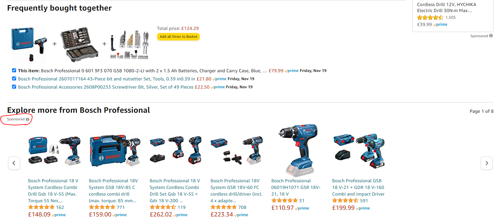
  • Became famous because of market basket analysis.

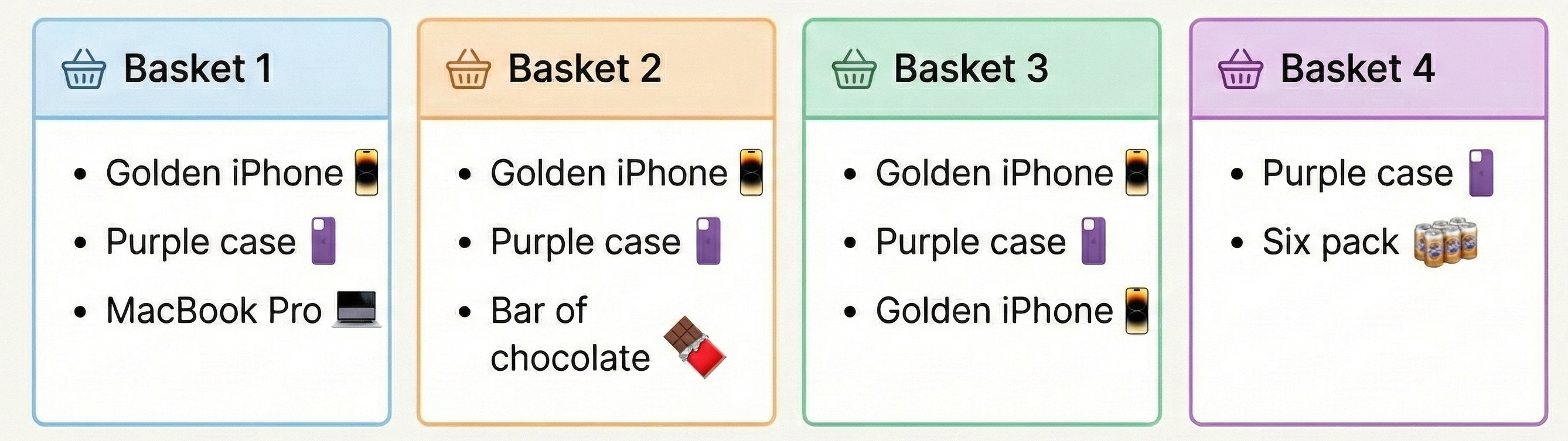
Example

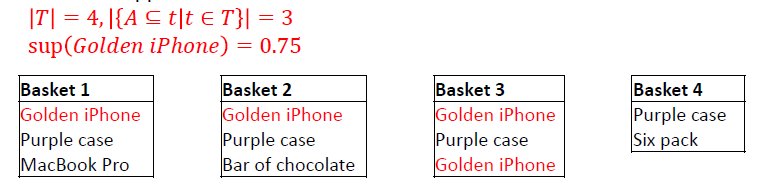
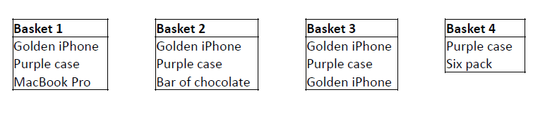
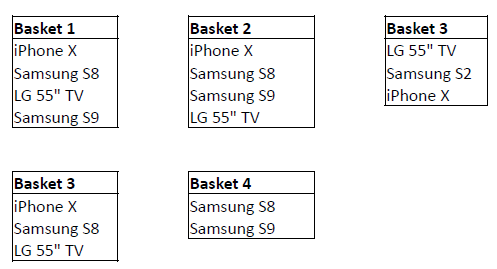
• Example: We have 4 Baskets

Finding Association Rules

• Association Rules:
  • Defined through an antecedent and consequent.
    • Both are subsets of \(I\).
  • Antecedent implies the consequent.
    • Example: Beer \(\rightarrow\) Diapers.
  • Calculated over transactions \(T\).
    • Represented as baskets.
  • Measuring Their Impact: Support, Confidence, Lift

Measuring Impact: Support

• Support: The number of times \(A\) appears among the transactions. \[ sup(A) = \frac{|\{A \subseteq t | t \in T\}|}{|T|} \]

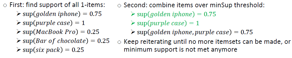
• Example: Calculate the support of Golden iPhone.

• Support: The number of times \(A\) appears among the transactions. \[ sup(A) = \frac{|\{A \subseteq t | t \in T\}|}{|T|} \]

• Example: Calculate the support of Golden iPhone.

Measuring Impact: Confidence

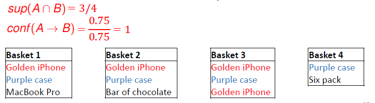
• Confidence: The number of times both itemsets occur together given the occurrence of \(A\). \[ conf(A \rightarrow B) = \frac{sup(A \cap B)}{sup(A)} \]

• Example: Calculate the confidence of Golden iPhone \(\rightarrow\) Purple Case.

• Confidence: The number of times both itemsets occur together given the occurrence of \(A\). \[ conf(A \rightarrow B) = \frac{sup(A \cap B)}{sup(A)} \]

• Example: Calculate the confidence of Golden iPhone \(\rightarrow\) Purple Case.

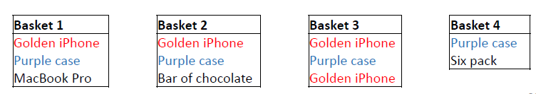
Measuring Impact: Lift

• Lift: The support for both itemsets occurring together given they are independent. \[ lift(A \rightarrow B) = \frac{sup(A \cap B)}{sup(A) \times sup(B)} \]

• Example: Calculate the lift of Golden iPhone \(\rightarrow\) Purple Case.

• Lift: The support for both itemsets occurring together given they are independent. \[ lift(A \rightarrow B) = \frac{sup(A \cap B)}{sup(A) \times sup(B)} \]

• Example: Calculate the lift of Golden iPhone \(\rightarrow\) Purple Case.

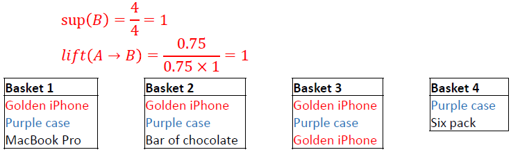
Lift value: example 1

\[ lift(A \rightarrow B) = \frac{sup(A \cap B)}{sup(A) \times sup(B)} \]

• Interpretation:
  • If lift > 1: Indicates both items are dependent on each other.
  • If lift = 1: Indicates both items are independent.
  • If lift < 1: Items are substitutes for each other.

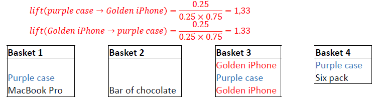
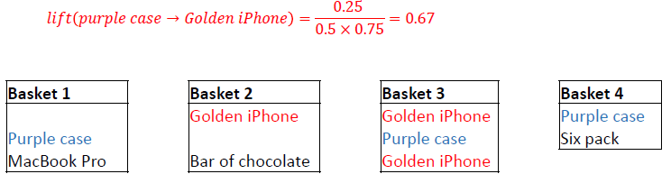
Lift value: example 2

\[ lift(A \rightarrow B) = \frac{sup(A \cap B)}{sup(A) \times sup(B)} \]

• Interpretation:
  • If lift > 1: Indicates both items are dependent on each other.
  • If lift = 1: Indicates both items are independent.
  • If lift < 1: Items are substitutes for each other.

A-Priori Algorithm

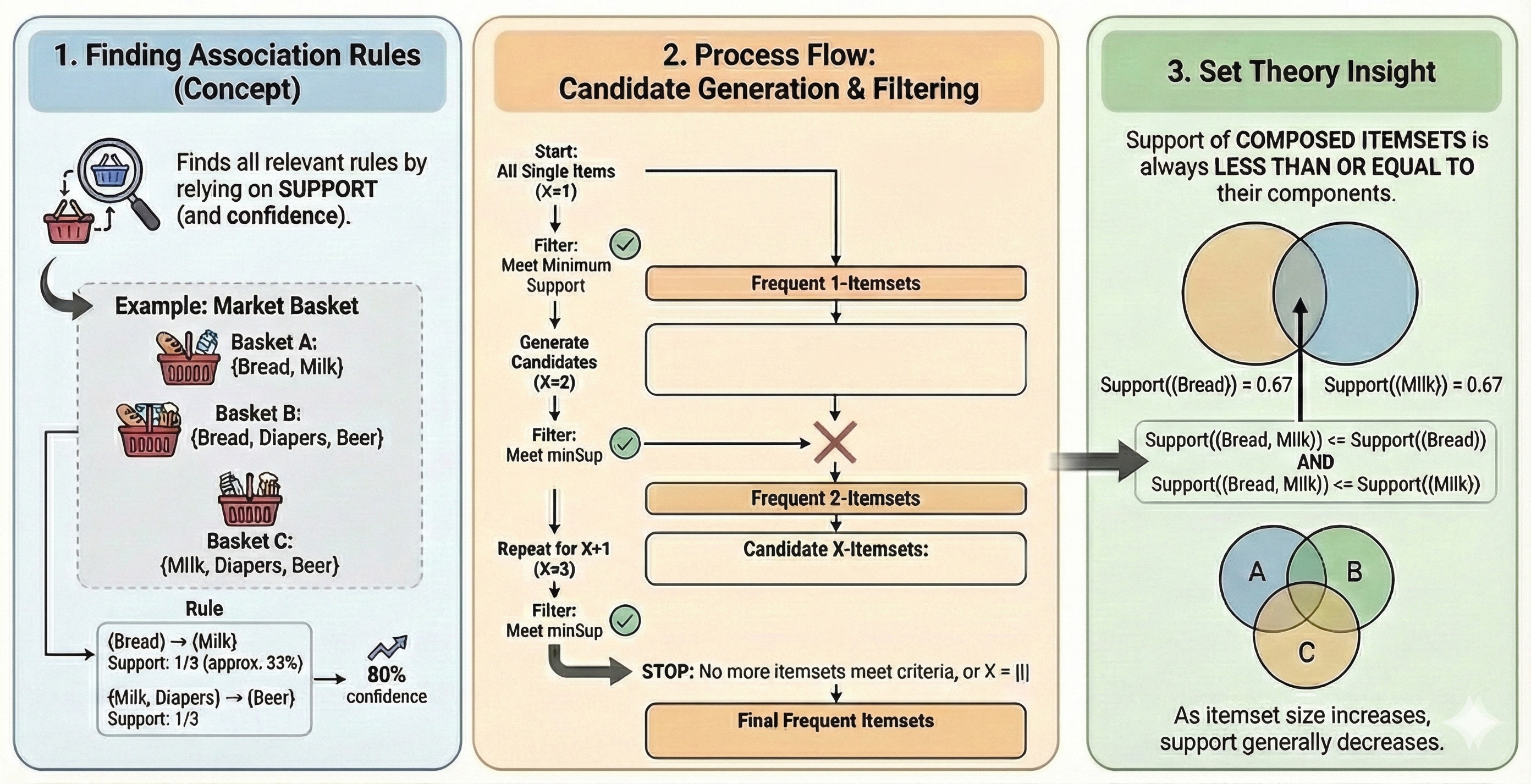
A-Priori Algorithm: Example

• A-Priori Algorithm Example (minSup 50%):

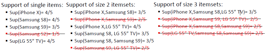
A-Priori Algorithm: Exercise

• Use the A-Priori Algorithm to find the frequent itemsets in the given transaction list.
• Minimum Support (minSup) = 60%.

Go to Wooclap

A-Priori Algorithm: Solution

• Minimum Support (minSup) = 60%.

Recommendation Systems

📊 Quick Poll: How Do They Know?

Wooclap Question

Go to wooclap.com and enter code: RMBELP

How do you think Netflix/Spotify know what to recommend?

• A. They read your mind
• B. They look at what similar users liked
• C. They analyze content features
• D. Random suggestions

🎯 The Answer: B (mostly!)

Collaborative Filtering: Find users like you, recommend what they liked. This is the core idea we’ll explore today.

The Recommendation Challenge

Think About It

ShopSocial has:

• 100,000 customers
• 50,000 products
• Each customer has bought ~20 products on average

That means 99.96% of the utility matrix is empty! How do we make recommendations with so little data?

Recommendation Systems

• Finding similar items to what people like:
  • Based on previous searches/purchases of others:
    • Collaborative filtering-based recommendation systems.
  • Based on items similar to the main interests of the user/buyer:
    • Content-based recommendation systems.
• Examples:
  • “Frequently bought together” on Amazon.
  • “Product related to this item” on virtually every webshop.

Example

Basics

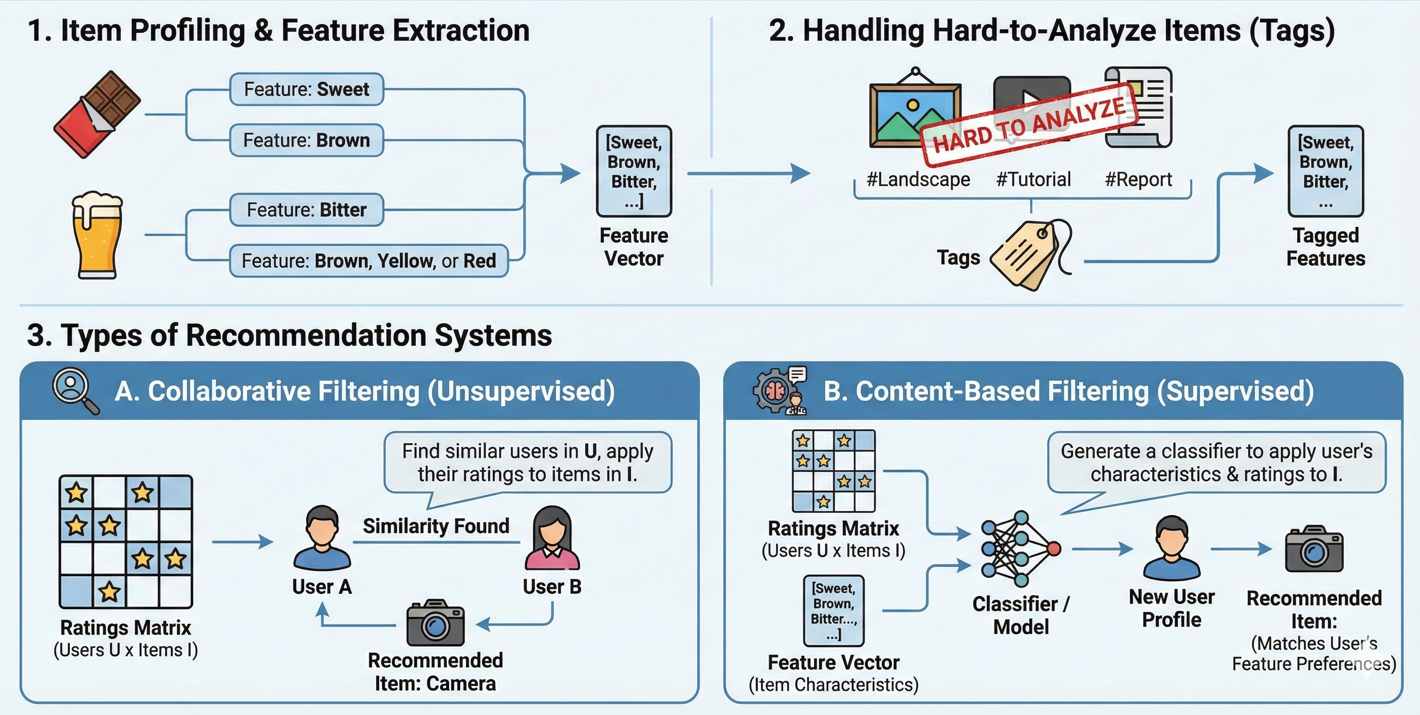
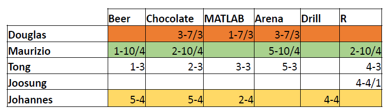
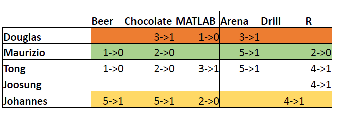
Representation: Utility Matrix

• Utility Matrix: Describes the relationship between users and items.

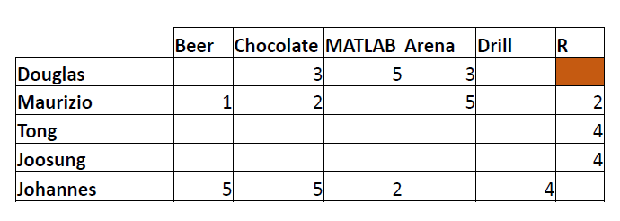
Question: Does Douglas like R?

Collaborative Filtering

• Collaborative Filtering:
  • Connecting users through similarity in items: User-to-user.
  • Connecting items through similarity in users: - Item-to-item.

Similarity Measures

• Jaccard Similarity (co-occurrence-based): \[ J(X, Y) = \frac{|X \cap Y|}{|X \cup Y|} \]
• Cosine Similarity (vector-based): \[ cos(\theta) = \frac{X \cdot Y}{\|X\| \|Y\|} = \frac{\sum_{i=1}^n x_i y_i}{\sqrt{\sum_{i=1}^n x_i^2}\sqrt{\sum_{i=1}^n y_i^2}} \]
• Pearson Correlation (not commonly used): \[ r_{X Y}=\frac{n \sum x_{i} y_{i}-\sum x_{i} \sum y_{i}}{\sqrt{n \sum x_{i}^{2}-\left(\sum x_{i}\right)^{2}} \sqrt{n \sum y_{i}^{2}-\left(\sum y_{i}\right)^{2}}} \]

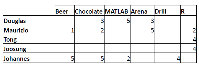
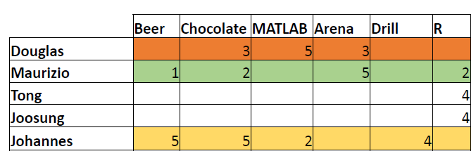
Similarity Measures: Example

Similarity Measures: Exercise

Question:

• Find the similarity between Douglas and Maurizio.
• Find the similarity between Johannes and Maurizio.
• What product(s) would you recommend for Maurizio?

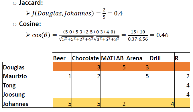
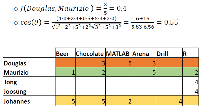
Similarity Measures: Q1 Solution

Q1: Find similarity between Douglas and Maurizio.

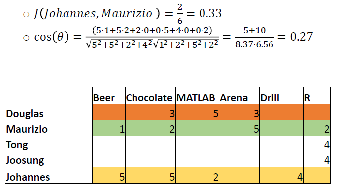
Similarity Measures: Q2 Solution

Q2: Find similarity between Johannes and Maurizio.

Similarity Measures: Q3 Solution

Question 3: What product(s) would you recommend for Maurizio?

• Recommendation Based on Similarity:
  • Highest similarity with Douglas.
  • Not previously acquired products that Douglas likes: MATLAB.

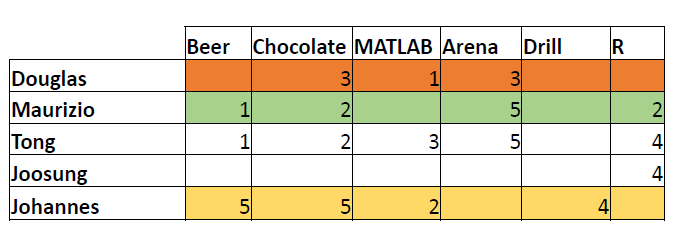
Similarity Measures: Q3+

Question 3+: What product(s) would you recommend for Maurizio now?

• Highest similarity with Douglas and Tong.
• Average rank of MATLAB:
  • For Douglas: Last 1 over 3 items; For Tong: Top 3 over 5 items.
  • Average ranking: Less than the middle.
  • Conclusion: No recommendation.

Other Actions: Cut-off

Other actions to improve results:

• Rounding, for example, cut-off at 3.

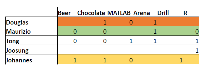
Other Actions: Cut-off (cont.)

Other actions to improve results:

• Rounding, for example, cut-off at 3.

Other Actions: Normalisation

Other actions to improve results:

• Subtract average of users’ rating from all ratings
• Turn low ranks into negative numbers and vice versa
• Bigger difference in similarity scores

Other Approaches

• Collaborative Filtering Alternatives:
  • Other approaches:
    • Cluster groups.
    • Find people in social networks with similar interests.
      • Relationships indicate relatedness.
      • Note that collaborative filtering is already a form of this.

Summary and Next Steps

📝 Quick Quiz: Test Your Understanding

Question	Your Answer
1. K-means requires specifying ___ in advance
2. VADER is designed for analyzing ___ text
3. Support measures how ___ an itemset appears
4. Lift > 1 indicates items are ___
5. Collaborative filtering finds similar ___

Answers:

1. K (number of clusters)
2. Social media
3. Frequently
4. Dependent/associated
5. Users (or items)

Key Takeaways

Clustering (Review):

• Groups similar items without labels
• K-means, Hierarchical, GMM, DBSCAN
• Used for customer segmentation (RFM)

Sentiment Analysis:

• Determines emotional tone of text
• Lexicon-based: count positive/negative words
• VADER: handles social media slang
• LLMs: flexible, contextual analysis

Frequent Itemset Analysis:

• Finds items that occur together
• Support, confidence, lift metrics
• A-Priori algorithm for efficiency

Recommendation Systems:

• Collaborative filtering: similar users/items
• Utility matrix representation
• Jaccard & Cosine similarity measures

Looking Ahead

Next Week: Ethics in Social Network Analytics

The techniques we learned today raise important questions:

• Sentiment Analysis: Can models be biased against certain groups?
• Recommendations: Do filter bubbles limit user exposure?
• Customer Profiling: What are the privacy implications?

We’ll explore:

• GDPR and privacy regulations
• Algorithmic fairness and bias
• EU AI Act and ethical frameworks

Questions?

Thank you!

Dr. Zexun Chen

📧 Zexun.Chen@ed.ac.uk

Office Hours: By appointment

Next Week: Ethics in Social Network Analytics