


Code
import networkx as nx
import plotly.graph_objects as go

# Create a Watts–Strogatz small-world network
G = nx.watts_strogatz_graph(n=30, k=4, p=0.1)

# Calculate a 3D layout for the nodes
pos_3d = nx.spring_layout(G, dim=3, seed=42)

# Extract node coordinates
x_nodes = []
y_nodes = []
z_nodes = []
for node in G.nodes():
    x_nodes.append(pos_3d[node][0])
    y_nodes.append(pos_3d[node][1])
    z_nodes.append(pos_3d[node][2])

# Build edge coordinate lists for Plotly
edge_x = []
edge_y = []
edge_z = []
for edge in G.edges():
    x0, y0, z0 = pos_3d[edge[0]]
    x1, y1, z1 = pos_3d[edge[1]]
    # Plotly needs a break (None) to start a new line for each edge
    edge_x += [x0, x1, None]
    edge_y += [y0, y1, None]
    edge_z += [z0, z1, None]

# Create a Plotly trace for edges
edge_trace = go.Scatter3d(
    x=edge_x, y=edge_y, z=edge_z,
    mode='lines',
    line=dict(color='lightblue', width=2),
    hoverinfo='none'
)

# Create a Plotly trace for nodes
node_trace = go.Scatter3d(
    x=x_nodes, y=y_nodes, z=z_nodes,
    mode='markers',
    marker=dict(symbol='circle', size=5, color='pink'),
    text=[f"Node {n}" for n in G.nodes()],
    hoverinfo='text'
)

# Combine the traces into a figure
fig = go.Figure(
    data=[edge_trace, node_trace],
    layout=go.Layout(
        title="Small-World Network in 3D (Plotly)",
        showlegend=False,
        scene=dict(
            xaxis=dict(showbackground=False),
            yaxis=dict(showbackground=False),
            zaxis=dict(showbackground=False)
        )
    )
)

fig.show()
 Source:


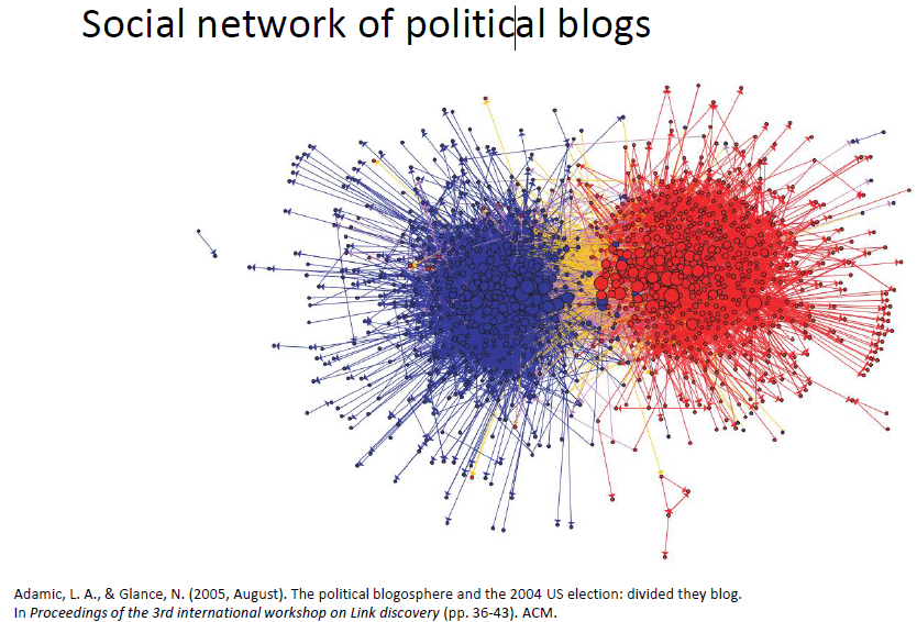
Social Media